Medians with Zero

Introduction

The median is a measure of central tendency that returns the middle value in a range of values as opposed to the mean, which returns the total of all values divided by the number of values. In Excel, there is the MEDIAN() and there is the AVERAGE() function. In addition, there are the AVERAGEA(), AVERAGEIF() and AVERAGEIFS() functions; but no such equivalents for the median.

There is always the problem of what to do with zero values or null values in a range when finding averages. The purpose of this post is to illustrate how we can use a combination of an array function and Power Query to deal with ranges of data that includes one or more zero (null) values.

Simple Example

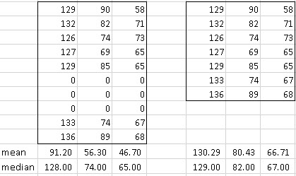
Consider the following table showing the mean and median from a selection of data from a much larger table and then see what happens when we reorganise that table to exclude zero values from our calculations:

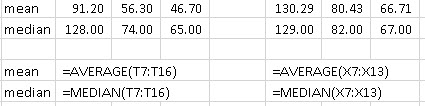
It helps us to see the formulas I have used in the mean and median calculations:

By leaving 0 or null entries in the data, we can get significantly different results from when we exclude them. What I mean is, a zero value or null value (empty cell) should not be included in the formulas because the cells are merely empty and they do not contain a value at all. I need to say, though, that if a cell really does contain a meaningful 0 value then leave it in the data to be evaluated.

Power Query (Get & Transfom)

Let’s create our Query now that will help us with the array formula that comes a little later.

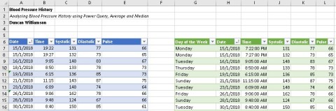
In the file that you can download from this page, click anywhere in the Excel table that I have already given the name bp_days.

Data tab ==> From Table/Range ==> this will open the Query Editor and you will see your Excel table in there in full:

Part of this exercise is to find the median values day by day and for that we need to create a Day of the Week column. Of course, you can also create a column for month, quarter … anything you like!

Right click on the Date column header and click Duplicate Column that wil give you a Date – Copy Column

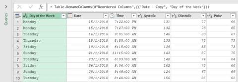
Click on the Date – Copy column ==> Transform Tab ==> Date ==> Day ==> Name of Day and that will transform your duplicate dates into Monday, Tuesday, Wednesday … Rename the column Day of the Week and right click, Move, To Beginning to move the column to the left.

To remove all of the null/zero rows, click on the Systolic column header down arrow and deselect null ==> OK. All of your empty cells have now gone.

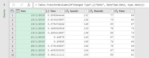
Time is shown as a decimal number. Look at the column header where you can see 1,2 Time … that confirms that it is a decimal number and not a time. Right Click on the header Change Type ==> Time.

Now click on the header ==> Transform Tab ==> Time ==> Time only. Done!

We have finished our Query and it should look like this:

I want my query next to my Excel table so I click the Home Tab ==> Close and Load down Arrow ==> Close and Load to… Existing Sheet cell E6 ==> OK.

Now you see this:

If you are happy to have your Query table on another worksheet just click Close and Load and it will do that for you.

Finding the Median Day by Day

We have already seen that the median function is really simple to use, =MEDIAN(T7:T16), for example. However, we want to find the median for each day of the week and for that we need to organise, essentially sort, the data and that means we need an ARRAY FUNCTION for that. For contrast, I am showing here how to find the mean values day by day and the median values day by day. These are the tables that we will create:

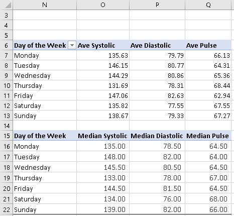
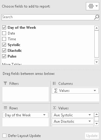
The first table, the Average or Mean values, are found by using a Pivot Table: I will not illustrate how I did that, beyond the following, which uses the Query as its data source:

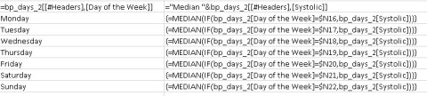
The table of median values in created by hand by using the following formulas … take your time and read them carefully. Then read my explanations that follow:

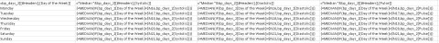
Click on the image to enlarge it but here are columns one and two enlarged for you:

Column 1 header is just a copy of the Column Header Day of the Week from the Query table. The rest of column 1 is a copy of days of the week from the Pivot Table.

The Column 2 header concatenates the word Median with the Systolic header from the Query table … similarly with columns 3 and 4.

The median systolic value for Monday comes from this ARRAY ENTERED formula:

=MEDIAN(IF(bp_days_2[Day of the Week]=$N16,bp_days_2[Systolic]))

Although it does not look like it, this really is an ordinary median formula but with an IF statement that gets the values rather than just naming a range.

1. Firstly, note that it also uses the Query table, with all null values removed
2. Secondly, it tells Excel to look for the name of the day in column 1, row by row, and then when it finds it, to aggregate all of the values it finds for Monday … Tuesday … etc and calculate the median for that day.
3. Thirdly, although IF statements should use this format =IF(logical test,[value if true],[value if false]), in this case there is no need for [value if false] because if it is false, IF essentially ignores  it and returns 0!

Having typed that formula in, don’t just type Enter or it will not work, press Ctrl and keep it pressed, then press Shift and kep it pressed and now press Enter and then let go of all three keys. The median Systolic vaue for Monday is 135.00 whereas the mean value is 135.63. You will often see array entering as CSE entered … Control+Shift+Enter

Conclusions

You are now an expert at finding the median values for a specif sub set of data. By using and IF statement inside a MEDIAN function, you are able to use a CSE function to do what would otherwide be impossible or long winded to do. By using the Power Query functionality, you have actually made life even easier for yourself.

By the way, assume you wanted to illustrate the median values for Monday at a certain time or Monday for a certain person (assuming we are given data for more than one person and their names are in a new column, Name, in our Excel table) and the names are shown in, say, column O of our output table, we would just need to extend our median function like this:

=MEDIAN(IF(bp_days_2[Day of the Week]=$N16,if(bp_days_2[Day of the Week]=$O16),bp_days_2[Systolic])))

You can try that for yourself.

Download my Excel file from here Please note, this file is already fully worked so if you do want to recreate my Query, be aware that you need to create a new one … median_array_function

In that Excel file you will also find these graphs, among others …

Duncan Williamson

6th December 2018