Flash Fill & Power Query

I came across the article Experts Share Their 10 Favorite Excel Functions today and in there you will find that 20 Excel MVPs have said what their favourite ten Excel functions are: take a look and learn what seems to be used most often. I downloaded the list so that I could refer to it in my work and I found I need to use as I found 87 unique functions being nominated:

• Flash Fill
• Power Query
• Pivot Table
• Slicer

You can download my Excel file from the link at the end of this post.

Flash Fill

The list is in this format:

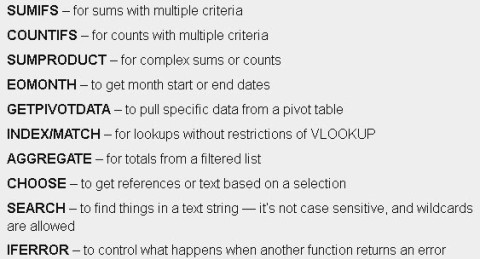
and when I pasted it into my worksheet I wanted to split out the name of the function from the rest of the cell contents. Not too long ago this could have been time consuming, meaning that we would have to use LEFT() and MID() and possibly RIGHT() as well. In this case, I invoed Flash Fill:

in the column to the right of the column of functions and explanations, I started by typing SUMIFS() then Enter, in the next row I typed COUNTIFS(). I didn’t see Flash Fill doing anything so I went to Data … Flash Fill and it told me nothing had happened yet. So I typed the next name, SUMPRODUCT and sure enough, Excel then split out the functions for meALMOST entirely. There were about ten cells in which Flash Fill was not so sure so I edited them manually and that gave e my complete list.

I should add that some MVPs presented two or more functions together like this: IF, AND; others did it this way, IF/AND. I standardised everything to make them look like IF/AND … and that helped a lot.

At the end of those few minutes I had extracted my list of functions. However, there were rows like this: LEFT/RIGHT/MID. I needed to split those too and decided I would split them into rows. I needed Power Query for that!

Power Query

This screenshot shows the problem and the solution:

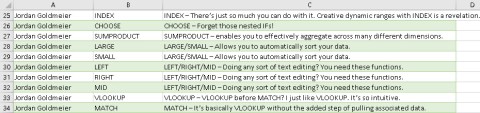
In column C, eg row 28, you can see LARGE/SMALL, in which an MVP has listed two, sometimes more than two, functions together. As I mentioned, I standardised the presentation of these functions and got Power Query to split the function column, B, into rows so that LARGE/SMALL became LARGE on row 28 and SMALL on row 29: notice how cell C28 is repeated in cell C29 in full.

How did I split the cells?

I had created an Excel Table to hold the data:

MVP’s name

The functions, split using Flash Fill as described above

The function/description/justification

Data … From Table/Range …

In PQ, Highlight the Fuction(s) column … Home … Split Column … PQ suggests that the delimiter is / which it then says you can use to split the column once, using the left most / or once using the right most / and at every instance of / … I chose at every instance

Click on Advanced Options now … Rows … OK

PQ now shows your complete list with every chosen function on its own line …

I had my completed list now and moved on to the final stage

Pivot Table

I wanted to determine just how many unique functions the MVPs had chosen and which were the most popular or frequently chosen functions. Easy peasy now:

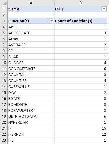
My pivot table has

MVP names in the Filter Area

Function(s) in the Rows area

Count of Function(s) in the Values area

and it looks like this, in part, in alphabetical order:

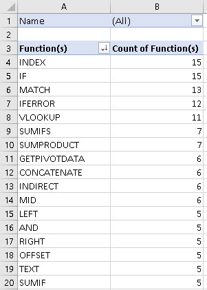
The top functions are:

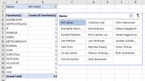
Slicer

Finally, I added a slicer for the MVP names and this is what that does for Bill Jelen’s selections:

Download my Excel file here top_10_functions_mvp

Duncan Williamson

24th June 2017