When I run an Excel course or finance course that includes an element of Excel, I stress the need for and use of templates. For example, imagine we are discussing ratio analysis: one of the best things we can do is to create a ratio analysis template that takes all of the data from our source/work sheet/database and automatically calculates a series of ratios for us.
We might have data for one or more companies for
- the income statement
- the balance sheet and
- the cash flow statement and
we could find ratios for
- profitability
- asset usage and
- liquidity
One of the key features of such a template or ratio analysis model is that the inputs have to be created carefully so that whatever you put in there can be translated seamlessly by Excel into the ratios you want. This can be a big problem and what follows demonstrates the problem and one solution to it.
In the Excel file that accompanies this page you will see two sets of Income Statement (IS) data for two companies. The two companies I chose to examine are
- SUNEDISON INC
- WORTHINGTON INDUSTRIES INC
I chose these companies almost at random and for no reason other than that their income statements were not identical.
Starting with Sunedison Inc, I copied and pasted ten years’ worth of IS data into a new workbook: I copied it from http://www.morningstar.com. I did the same for Worthington Industries Inc
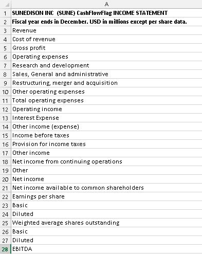
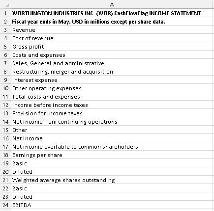
Take a look at the two IS account names columns now:
- notice that Sunedison ends on row 28 while Worthington ends on row 24: immediately we can see something is different
- secondly, notice that after the first few lines, again, we start to see differences. For example, Sunedison has Research and development expenses and Worthington does not
- then see that the order in which the account names are presented is not consistent: for example, interest expense is a lot lower down the IS for Worthington than it is for Sunedison.
Two Approaches
There are two sensible approaches to the problems I have just outlined but there are others!
Standardised IS and Template
In the Excel file you will see two tabs:
- SUNE_tidied
- WOR_tidied
What I did there was to standardise the layout of both IS, by moving things around and so on to ensure that both IS ended on line 28 with all account names on the same lines etc. Having done that, we can now create a ratio analysis template, as you can see on the template tab:
In cell O4 we see the basic formula for the gross margin ratio =C5/C$3*100 and that’s all we need: fill right and the whole of that row is complete. Repeat for the other ratios.
This is fine, by the way, as it does what we want it to but do notice the empty rows for the research and development and operating income data: empty for Worthington, as shown here.
Use a VLOOKUP Approach
Using what I am calling the VOOKUP approach allows you to do one labour saving thing: do nothing! That is, there is no need to do any standardisation or any preparation except of the ratio table itself. This means that we can take the IS data from http://www.morningstar.com and paste it into the non standardised template tab and it will work even though there are inconsistencies of data and layout.
For Worthington
Not convinced? Take a look at the two tabs WOR_ratios and SUNE_ratios and see how I have kept the data in their raw and unedited format and yet the template can find and evaluate the ratios we need: providing the data are in the IS. For Sunedison, then,
VLOOKUP Formulas
Here is the VLOOKUP() formula I used, from the WOR_ratios tab, cell O4
=IFERROR(VLOOKUP($N4,inc_st,O$1+1,0)/C$3*100,”-“)
That for the gross profit margin for 2014 and you can fill right with that and then create the quivalent formula for the other ratios.
Conclusions
The VLOOKUP solution here is very clever and it means that if your focus is on the output, the ratios, not the data or the IS, then this approach is ideal. Just make sure the spellings of the account names are the same as the spellings in the VLOOKUP formula and that’s all you need to worry about.
Here is the Excel file: sune_wor_vlookup_solution
Duncan Williamson


