After a delay of about a week, here is one of the articles I have been promising you on business intelligence.
Forecasting in Excel 2016
Forecast Sheet
I announced the other day that I would be discussing Business Intelligence in Excel and here is the first of those pages. In truth, I did not intend to write on this forecasting topic but then again, I didn’t have Excel 2016 when I said what I said!
In Excel 2016 they have included a new feature called Forecast Sheet and what they have done is to combined What if Analysis with the Forecast Sheet and combine them under the heading Forecast on the Data Tab:

Excel 2016 Introduces New Forecasting Functions
Here are the three new forecasting functions used in the example that I used to create this page.
- ETS
- ETS.CONFINT
- ETS.STAT
In the example I have used here, I just put the sales, total assets and net income data for amazon.com on three separate worksheets and then having clicked somewhere on the appropriate table, clicked Forecast Sheet and it opens up this dialogue box:
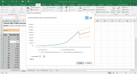
On that box you can see it has automatically drawn a line chart but you can change it to a column chart by clicking on its own icon in the top right corner.
It also tells you that it has made a forecast of periods 23 to 28: the actual data relate to periods 1 to 22 … you can change this if you want
It tells you the 95% (this is the default) confidence intervals for the forecasts too … again you can change this.
To make the changes I have mentioned, click on the arrow next to where it says Options in the bottom left hand corner of the Forecast Sheet dialogue box and now you will see several additional options. I have highlighted n the screenshot that follows where to make changes to
The type of graph shown
- How many periods to forecast
- The confidence level
- Whether to include forecast statistics
- And a few more that I have not highlighted

Change the
Forecast End to, say, 25 and see how the graph changes … you can change it back to 28
- Graph to a column graph … which do you prefer? … leave it or change it back
- Confidence level from 95% to 99% and watch what happens in the forecast area … change it back to 95% so you can compare it to mine
Select to include the forecast statistics and see what you get when you click: leave this selected for this demonstration! Click Create in the bottom right hand corner.
This is what I got:
Excel created what I am calling a forecast sub table below the table of raw data and in that sub table you will find:
- The forecasts for the periods 23 to 28
- The 95% Lower Confidence Bound (Net Sales $m)
- The 95% Upper Confidence Bound (Net Sales $m)
Unlike many functions built into the Data Analysis ToolPak for example, the Forecast Sheet includes the formulas it uses for the forecasts and the confidence intervals, as follows and here we see two functions that are new to Excel 2016:
Forecasts =C24 =FORECAST.ETS(A24,$B$2:$B$23,$A$2:$A$23,1,1)
Lower Confidence Bound = D24 = =C24-FORECAST.ETS.CONFINT(A24,$B$2:$B$23,$A$2:$A$23,0.95,1,1)
Upper Confidence Bound = E24 = =C24+FORECAST.ETS.CONFINT(A24,$B$2:$B$23,$A$2:$A$23,0.95,1,1)
The syntax of these functions is:
=FORECAST.ETS(target_date,values,timeline,[seasonality],[data_completion],[aggregation]))
=FORECAST.ETS.CONFINT(target_date,values,timeline,[confidence_level],[seasonality],[data_completion],[aggregation]))
FORECAST.ETS
From Excel’s Help File: Calculates or predicts a future value based on existing (historical) values by using the AAA version of the Exponential Smoothing (ETS) algorithm. The predicted value is a continuation of the historical values in the specified target date, which should be a continuation of the timeline. You can use this function to predict future sales, inventory requirements, or consumer trends.
This function requires the timeline to be organized with a constant step between the different points. For example, that could be a monthly timeline with values on the 1st of every month, a yearly timeline, or a timeline of numerical indices. For this type of timeline, it’s very useful to aggregate raw detailed data before you apply the forecast, which produces more accurate forecast results as well.
FORECAST.ETS.CONFINT
From Excel’s Help File: Returns a confidence interval for the forecast value at the specified target date. A confidence interval of 95% means that 95% of future points are expected to fall within this radius from the result FORECAST.ETS forecasted (with normal distribution). Using confidence interval can help grasp the accuracy of the predicted model. A smaller interval would imply more confidence in the prediction for this specific point.
In both cases, we use the options/arguments in this way:
- target_date: this is the forecast date/period for the current cell
- values: the range of raw or actual values on which the forecast is based
- timeline: the dates or range of dates relating to the raw data
seasonality: seasonal or non seasonal data … Optional. A numeric value. The default value of 1 means Excel detects seasonality automatically for the forecast and uses positive, whole numbers for the length of the seasonal pattern. 0 indicates no seasonality, meaning the prediction will be linear. Positive whole numbers will indicate to the algorithm to use patterns of this length as the seasonality. For any other value, FORECAST.ETS will return the #NUM! error. Maximum supported seasonality is 8,760 (number of hours in a year). Any seasonality above that number will result in the #NUM! error.
Look at the formulas Excel 2016 has created to see how it is using these arguments.
data_completion in both cases allows us to chose from two options
0 missing data treated as zero
1 auto completion uses linear interpolation
Aggregation From Excel’s Help File: Optional. Although the timeline requires a constant step between data points, FORECAST.ETS.CONFINT will aggregate multiple points which have the same time stamp. The aggregation parameter is a numeric value indicating which method will be used to aggregate several values with the same time stamp. The default value of 1 (Excel’s Help File says 0 will use AVERAGE but the list starts with Average taking a value of 1), while other options are SUM, COUNT, COUNTA, MIN, MAX, MEDIAN: see the list the follows.
In both cases allows us to choose from seven options
- AVERAGE
- COUNT
- COUNTA
- MAXIMUM
- MEDIAN
- MINIMUM
- SUM
Note: Excel did not set an aggregation level in my example.
The confidence_interval argument only applies to the CONFINT version of te FORECAST.ETC function and we set that in the Forecast Sheet when we say what the confidence interval should be: remember the default is 95% but you can change it as we have already seen.
The Statistics table is based on this function, again new to Excel 2016:
FORECAST.ETS.STAT
From Excel’s Help File: Returns a statistical value as a result of time series forecasting. Statistic type indicates which statistic is requested by this function.
Syntax
FORECAST.ETS.STAT(values, timeline, statistic_type, [seasonality], [data_completion], [aggregation])
You only get these statistics if you tick the box to Include forecast statistics.
In a separate table to the right of the raw data and the graph there is the Statistics table that includes the statistic_type:
- …Alpha parameter of ETS algorithm Returns the base value parameter: a higher value gives more weight to recent data points.
- … Beta parameter of ETS algorithm Returns the trend value parameter: a higher value gives more weight to the recent trend.
- … Gamma parameter of ETS algorithm Returns the seasonality value parameter: a higher value gives more weight to the recent seasonal period.
- … MASE metric Returns the mean absolute scaled error metric: a measure of the accuracy of forecasts.
- … SMAPE metric Returns the symmetric mean absolute percentage error metric: an accuracy measure based on percentage errors.
- … MAE metric Returns the symmetric mean absolute percentage error metric: an accuracy measure based on percentage errors.
- … RMSE metric Returns the root mean squared error metric: a measure of the differences between predicted and observed values.
- … Step size detected Returns the step size detected in the historical timeline: in my example, Eel did not include this statistic type. It would have shown a value of 1 had it been included because the timeline increases one period at a time.
Final Output

Conclusions
I am sure this is a welcome addition the functionality of Excel although I have yet to get fully to grips with the Statistics Table. There is a lot here that has been automated yet there is scope for choice of confidence intervals, forecast end period and so on.
As you can see with the forecast of amazon.com sales, Forecast Sheet gives us a set of answers but they don’t look to be too good. However, in a year’s time we might well see that the company’s ales really have dropped from $107 billion to $85.3 billion as Excel is suggesting it will.
Duncan Williamson
