Creating and Using a Scroll Bar

Scroll Bars in Excel

I have used Excel for mac²⁰¹¹ to demonstrate a spreadsheet from my Manpower Planning friend Tony that finds appraisal results and values. Excel 2010 copes equally well with what you are about to read about but the scroll bars look nicer on the mac!

One of the features Tony wanted me to include was what he called sliders: Excel users call them scroll bars or scrollbars.

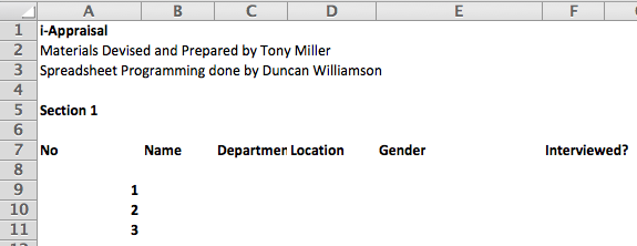
What follows is just PART of the work sheet I created: the work sheet starts here with some basic data on the employee being appraised

Tony and Duncan did this!

In the third section of the work sheet (yes, I’ve missed out section 2!) we see the scroll bars … just use the left mouse button to move the sliders left or right to decrease or increase the value from the appraisal for the appropriate measure in column F, the summary values in rows 25, 30 and 35 are found automatically by formula, as is the total in row 40:

Tony and Duncan did this too

The next screen shot is a repeat of the previous one except that I have moved the scroll bars around so that you can see what it looks like when different employees’ results are displayed:

Tony and Duncan did this as well!

How did we do this?

• Click on the Developer tab
• Click on scroll bar and then draw it on your work sheet how you would like it to appear: how and what size
• Right click your new scroll bar and click Format Control and this appears (Excel mac²⁰¹¹)

How to set up a croll bar

In this case the values to use are:

• the current value is 0 … in some cases this might not be true, it depends which cell you have selected when you create the scroll bar … change it to WHATEVER value you want … 0 is fine here
• we want the maximum value to be 100 … in your case that might not be true
• we want the incremental change to be 1 … that is, if you use the Windows version of Excel, click on the scroll bar arrows and the bar moves one number at a time
• leave the page change at 10 … if you click in a scroll bar next to the slider rather that on the scroll bar arrows, your numbers change by 10 not incrementally one by one … change it to 3 or 5 of 20 as you wish
• Finally, click on the cell link: this is the cell where your appraisal score will appear … in the section 3 screenshot we would choose cell link F26 for the score for “Delivering results and quality”
• Now click away from the scroll bar to deselect it and then use it!

Repeat for every scroll bar you want:

• arrange them as YOU want … remembering who will use you work and how
• you can only use integers for the values to put into the scroll bars minimum value, maximum value and incremental value, that is. If you want decimals … well, see if you can work out how to make that work … it’s not too difficult!

Well, that’s it! A really useful thing to know!

One more thing, what we have created is a form based scroll bar not an ActiveX scroll bar … not that it really matters here!

ADDITIONAL Help

Following on from a comment I have added the following together with a file that you should find helpful. Thanks to Blog Member azamtokhi for encuraging me to add these! This relates to a NEW example.

Scroll Bar

The purpose of the scroll bar can be to get a piece of information and use that to create the kind of table we have just seen under the revious example.. It could be just to get one piece of information or many. It could be to help us to control graphs or dashboards as we will see later.

In any case, this is how scroll bars work.

Click on Developer Tab, Controls, Insert and click on Scroll Bar (Form Control) which is third from the left on the second row.

You cursor will change to cross hairs and you can draw the outline and size of your Bar wherever you want now: in this case the bars look much better drawn vertically rather than horizontally. In our case we drew it to cover the range A8:A14 and made it just wide enough to look pleasing, which is where it stays now.

Right click on the Scroll Bar and select Format Control at the bottom of the menu you will see.

In the dialogue box that opens now make these changes:

Make the

• Current value … leave that alone as Excel keeps track of that
• Minimum Value in this case is 1
• Maximum value in this case is 8
• The incremental change is 1: this tells Excel how many to add to or subtract from the number in the cell link when you click the Scroll Bar arrows once: top arrow decreases, bottom arrow increases
• The Page change is 1: when you click on the Scroll Bar between the arrows, Excel will add to or subtract 1 from the number in the Cell link depending on where you clicked it
• The Cell link is I24: this does the same as it does with the Combo Box but we put it in its own cell to stop any conflicts with the Combo Box
• Click OK

Here is the dialogue box BEFORE any changes:

Click away from your Scroll Bar now to deselect it and then click on its down arrow. In this case there is nothing to see: you don’t see aaaa, bbbb … yet, unlike the Combo Box. However, to see what we need, we now do exactly what we did with the Combo Box except in a different table. Again, the Cell link is the key to using the scroll Bar: click somewhere on the scroll bar and the number in cell I24 changes.

The main purpose of something like a Scroll Bar is to use it! In this case we will use this Bar, via the number in cell I24 to populate the range B9:F9:

Copy the column headers from H15:L15 … Name, ID etc … into B8:F8

Enter this formula in cell B9: =VLOOKUP($H24,$G$16:$L$23,H14,0)

This formula says

• look in cell I24 and see what number is there
• remember that number and look for it in the first column of G16:L23
• when you find that number move across to column two of that range and tell cell B9 what it found there
• in this case, since the number in cell I24 is 1, the answer for B9 is aaaa

Make a note of all of the $ in the formula and the cell references and then fill the formula right to F9

This is what it should say when the number in cell I24 shows 1:

Name	ID	Date Joined	Texture	Plant
aaaa	489	1/1/2013	soft	grass

When the number in cell I24 says 5:

Name	ID	Date Joined	Texture	Plant
eeee	138	6/5/2013	wooden	flower

Exercise for you

Since Combo Boxes and Scroll Bars are rather more complex that data validation, try these exercises.

1 Use your Combo Box to create an output table like this:

Name	aaaa	ID	100
Date Joined	1/1/2013	Texture	soft
Plant	grass

2 Use your Scroll Bar to create the following table ON A NEW WORKSHEET, call the worksheet forms_2.

To complete this exercise you should use an ARRAY ENTERED TRANSPOSE formula to create the headings in column B and you should use additional column heading controls in your VLOOKUP() formula. Make the Page Change value in the Scroll Bar dialogue box equal to 3. Add some Alt text: make it clear and understandable! Finally, to avoid conflict with your other Scroll Bar in this work book, make forms!I25 your cell link.

Test your results!

Here is the Excel file for you to download and work on combo_scroll

Duncan Williamson